From Obscurity to Ubiquity: The 50-Year Journey of Bayesian Optimization
Introduction
Bayesian Optimisation achieved widespread adoption in the 2010s after nearly four decades of theoretical development, driven by the need to find the optimal hyperparameters in large neural networks. Recently, it has found an application in the manufacturing as well as chemical industry, where the output of a process is usually expensive or time-consuming. The popularity increased not because there was a sudden improvement in theory, but rather due to the increase in computational infrastructure and a need to find the optimum of black-box functions in a limited amount of time and/or resources.
How it started?
The story has twin origins: in 1951, Danie Krige developed spatial prediction methods in South African gold mines, while in 1964, Harold Kushner independently created sequential design algorithms at Brown University, both solving the same mathematical problem in wildly different contexts. These parallel threads would converge through Jonas Mockus’s Lithuanian school in the 1970s, accelerate with Jasper Snoek’s 2012 paper proving Bayesian Optimisation beats human experts at hyperparameter tuning, and culminate in today’s integration with large language models and autonomous laboratories. Along the way, Bayesian Optimisation’s trajectory illustrates how expensive blackbox optimisation problems, which were once rare curiosities in mining and control systems, became ubiquitous with the rise of machine learning, creating economic pressures that finally justified the method’s computational overhead. This narrative arc from theoretical elegance to practical necessity offers lessons for researchers wondering when their own algorithms might find their moment.
Krige and the Birth of Spatial Statistics (1951)
The story of Bayesian Optimisation does not begin in a university laboratory or a control systems department, but rather in the depths of South African gold mines. In 1951, Danie Gerhardus Krige, a mining engineer working in Johannesburg, confronted a problem that would unknowingly lay the groundwork for modern machine learning: how to estimate ore concentrations throughout a mine based on expensive, limited drill samples.
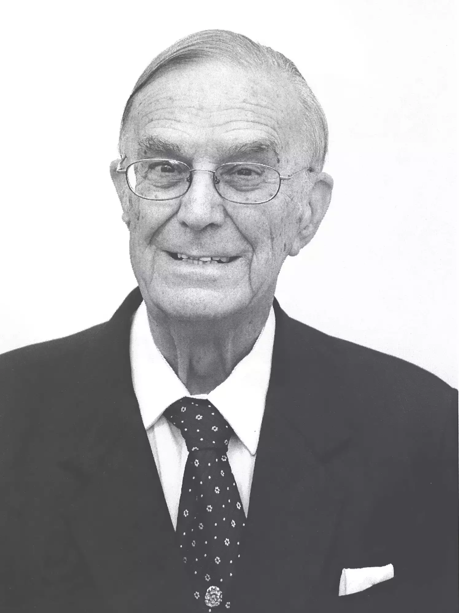
Krige’s master’s thesis addressed a challenge that mining companies faced daily: drilling for samples was costly and time-consuming, yet accurate estimates of gold grades across large volumes were essential for economically sound decisions. Traditional averaging methods failed catastrophically because they ignored a crucial property, i.e. spatial correlation. Ore grades at nearby locations tend to be similar, while distant samples are nearly independent.
The technique that would bear his name, Kriging, predicts values at unsampled locations using a weighted average of nearby observations: \[\hat{f}(x) = \sum_{i=1}^n w_i(x)y_i\]
But here’s the clever part: the weights wi(x)w_i(x) wi(x) aren’t arbitrary. They’re chosen to minimize prediction variance while ensuring the estimator is unbiased. This required modeling the spatial correlation structure through what Krige called a variogram, a function describing how similarity decreases with distance between sampling points.
Matheron’s Mathematical Formalization
Krige’s empirical methods caught the attention of French mathematician Georges Matheron, who spent the 1960s building a rigorous mathematical theory around spatial interpolation. In his seminal 1963 work, Matheron introduced the theory of random functions and proved something remarkable: under Gaussian assumptions, the Kriging predictor is equivalent to the conditional expectation of a random field given the observations.
Matheron’s formalization revealed that Kriging implicitly assumes:
- The unknown function \(f(x)\) is a realization of a Gaussian random field
- The covariance between function values depends on their spatial separation: \(Cov(f(x), f(x')) = k(x,x')\)
- Predictions should use the full conditional distribution given observed data
This probabilistic framework—treating unknown functions as random processes with correlation structures—would resurface in dramatically different contexts over the coming decades.
What Krige and Matheron had created was mathematically equivalent to what we now call Gaussian process regression, though that terminology wouldn’t emerge until decades later in the machine learning community. The posterior mean formula that appears in modern Bayesian optimization: \[\mu(x) = k(x,X)^T[K(X,X) + \sigma_n^2 I]^{-1}y\] is mathematically identical to Matheron’s Simple Kriging predictor under a zero or known mean assumption.
Yet this connection remained hidden for years. Kriging stayed confined to geostatistics, mining, and spatial analysis, while the ideas that would become Bayesian optimisation emerged independently in control theory and operations research. Kushner, working on sequential design in 1964, almost certainly had no knowledge of Krige’s mining work from 1951. The parallel evolution of nearly identical mathematical frameworks in completely separate fields speaks to the fundamental nature of the problem: how do you efficiently explore an expensive, uncertain function?
The prophetic beginnings: Kushner and the birth of sequential design (1964)
The intellectual foundation for Bayesian Optimisation emerged from an unlikely source: control systems engineering in the early 1960s. Harold Joseph Kushner, an applied mathematician at Brown University, confronted a deceptively simple problem that would define a new field. His 1964 paper “A New Method of Locating the Maximum Point of an Arbitrary Multipeak Curve in the Presence of Noise” in the Journal of Basic Engineering introduced what we now recognise as the first Bayesian Optimisation algorithm.
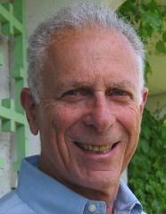
Kushner’s revoutionary insight was treating the unknown objective function as a realisation of a Wiener process(Brownian Motion), essentially placing a probabilistic prior over all possible functions.
For a one-dimensional function, consider searching for the maximum of an unknown function \(f(x)\) over an interval [a,b], Rather than assuming a deterministic form, Kushner modeled the function as having increments that follow a Wiener process. A standard Wiener process \(\mathbf{{W(t)}_{t\geq0}}\) has several key properties:
- Independent Increments: For any times \(0\leq s < t\), \(W(t) - W(s)\) is independent of all previous values
- Gaussian distribution: Each increment satisfies \(W(t) - W(s) \sim \mathcal{N}(0, t-s)\)
- Continuity: The paths \(W(t)\) are continuous in time
By treating the function values as following a stochastic process with these properties, Kushner could compute conditional probability distributions about where the maximum might be located based on noisy observations \(y_i = f(x_i) + {\epsilon}_i\) at sampled points where \(\epsilon \sim \mathcal{N}(0, \sigma^2)\) represents measurement noise.
Crucially, Kushner introduced the Probability of Improvement (PI) acquisition function, which explicitly balanced exploring uncertain regions against exploiting known good areas. The approach allows us to ask the question: given our current observations, at which location are we most likely to find a value better than our best observation so far?
In modern formulations using Gaussian processes(which became standard decades later), the PI acquisition function takes the elegant closed form: \[PI(x) = P(f(x) > f^* + \xi) = \Phi(\frac{\mu(x) - f^* - \xi}{\sigma(x)}) \] where:
- \(\mathbf{f^*} = max_{i=1,...,n}y_i\) is the best observed value so far
- \(\mathbf{\mu(x)}\) is the posterior mean prediction at location \(x\)
- \(\mathbf{\sigma(x)}\) is the posterior standard deviation representing our uncertainty in the predicted value
- \(\Phi(.)\) is the cumulative distribution function of the standard normal distribution
- \(\xi \geq 0\) is a small exploration parameter (often set to 0 or 0.01)
The next sampling point is chosen by maximising this probability \(x_{n+1} = \text{arg max}_x PI(x)\).
The beauty of this criterion is evident in its behaviour: PI increases both where the predicted mean \(\mu(x)\) is high (exploitation) and where uncertainty \(\sigma(x)\) is large (exploration), providing a principled balance between these competing objectives.
It is worth noting that while Kushner’s original 1964 work used Wiener processes, the formulation above evolved with the adoption of Gaussian processes in later decades, particularly through the work of Mockus in 1970s and Jones in 1990s, which we are going to discuss in the following subsections. But I hope you can see the importance of this formula towards finding the maximum or minimum of multimodal functions. It is extremely hard for models to not get stuck at a local maxima or minima, and thus, the introduction of an exploration term is extremely crucial.
The Lithuanian school and Expected Improvement (1970s)
While Kushner’s work remained largely confined to control theory circles, a parallel revolution emerged from an unexpected place: Soviet Lithuania. Jonas Mockus, working at the Institute of Mathematics and Informatics in Vilnius, would become the founder of modern Bayesian optimisation and the person who coined the term itself. His contributions, initially published in Russian and presented at Soviet-bloc conferences, established the theoretical foundations that remain standard even to this day.
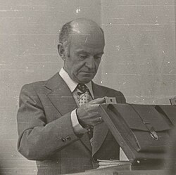
Mockus’ seminal 1974 paper “On Bayesian Methods for Seeking the Extremum” presented at the IFIP Technical Conference in Novosibirsk (published in Lecture Notes in Computer Science, Vol.27, Springer) introduced the Bayesian framework for global optimisation. But his most influential contribution came four years later. The 1978 paper with collaborators Vyatutas Tiesis and Antanas Žilinskas, “The Application of Bayesian Methods for Seeking the Extremum” in Dixon and Szego’s influential volume Towards Global Optimisation Vol. 2, introduced the Expected Improvement (EI) acquisition function.
The criterion elegantly solved the exploration-exploitation dilemma through a rigorous probabilistic framework. At the heart of the method lies the Gaussian Process (GP) model of the unknown objective function \(f(x)\). After observing function values \(y = [y_1, y_2, y_3,..., y_n]^T\) at locations \(X = [x_1, x_2, x_3,...,x_n]^T\), the GP posterior distribution at new point \(x\) is characterised by: \[\mu(x) = k(x, X)^T[K(X,X) + \sigma_n^2I]^{-1}y\] \[\sigma^2(x) = k(x,x) - k(x,X)^T[K(X,X) + \sigma_n^2I]^{-1}k(x,X)\] where \(k(x,x')\) is a covariance kernel function (commonly the squared exponential or the Matérn kernel), \(K(X,X)\) is the \(n\times n\) covariance matrix with entries \(K_{ij} = k(x_i, x_j)\), \(\sigma_n^2\) represents the observation noise, and \(I\) is the identity matrix. These formulas give us both a prediction \(\mu(x)\) and our uncertainty \(\sigma(x)\) about that prediction at any point.
Mockus’ key innovation was defining the improvement at any location \(x\) as: \[I(x) = max(f(x) - f^*, 0)\] where \(f^* = \text{max}_{i=1,...,n}y_i\) is the best value observed so far. The improvement is positive if we find something better than our current best, else it is 0. The \(Expected Improvement\) is then the expectation of this improvement under the GP posterior distribution. \[EI(x) = \mathbb{E}[max(f(x)-f^*, 0)]\] Since \(f(x)\) is normally distributed under the GP model with mean \(\mu(x)\) and variance \(\sigma^2(x)\), we can compute the expectation analytically. Let \(Z = \frac{\mu(x)-f^*}{\sigma(x)}\) be the standardised improvement. Then the expected improvement has the beautiful closed form: \[\text{EI}(x) = \begin{cases} (\mu(x) - f^*)\Phi(Z) + \sigma(x)\phi(Z) & \text{if } \sigma(x) > 0 \\ 0 & \text{if } \sigma(x) = 0 \end{cases}\] where \(\Phi(.)\) is the cumulative distribution function of the standard normal distribution and \(\phi(.)=\frac{1}{\sqrt{2\pi}}e^{-z^2/2}\) is its probability density function.
The formula’s elegance becomes clear when we examine its two terms:
- Exploitation term: \((\mu(x)-f^*)\Phi(Z)\) increases when the predicted mean \(\mu(x)\) exceeds the current best \(f^*\), weighted by the probability \(\Phi(Z)\) that we actually achieve improvement.
- Exploitation term: \(\sigma(x)\phi(Z)\) increases with uncertainty \(\sigma(x)\), encouraging sampling in regions where there is limited information.
To understand the interplay, note that: 1. When \(\mu(x) \gg f^*\), we have \(Z \gg 0\), so \(\Phi(Z) \approx 1\) and the exploitation term dominates 2. When \(\sigma(x)\) is large relative to \(|\mu(x) - f^*|\), the exploration term provides significant contribution
The next sampling point is selected by maximising the acquisition function: \[x_{n+1} = \text{arg}\max_{\{x \epsilon \mathcal{X}\}}EI(x)\] where \(\mathcal{X}\) is the search domain.
An useful enhancement includes an exploration parameter \(\xi \geq 0\): \[\text{EI}(x; \xi) = \begin{cases} (\mu(x) - f^* - \xi)\Phi(Z_\xi) + \sigma(x)\phi(Z_\xi) & \text{if } \sigma(x) > 0 \\ 0 & \text{if } \sigma(x) = 0 \end{cases}\]
The effect of Exploration Parameter in Expected Improvement
The visualization below brings Expected Improvement to life. Watch as the algorithm balances exploitation (sampling where it predicts low values) against exploration (sampling uncertain regions) to efficiently find the global minimum of \(f(x) = \sin(3x) + x^2 - 0.7x\).
How to Interact:
Iteration Slider: Step through all 20 iterations to see how the Gaussian Process posterior (left) learns the true function shape, while the Expected Improvement (right) identifies the most promising next sampling location. The blue shaded region shows the GP’s uncertainty, notice how it shrinks around observed points.
Exploration Parameter (ξ): This is where the magic happens. Adjust ξ in real-time to control the exploration-exploitation trade-off:
- ξ = 0.0: This is Pure Exploitation. It greedily samples where the GP predicts the lowest values. Fast but risky; may get trapped in local minima.
- ξ = 0.01 (default): This is a balanced approach, the algorithm requires slightly more predicted improvement before exploiting, encouraging modest exploration.
- ξ = 0.1-0.3: This is Aggressive Exploitation, it demands significantly better predictions before exploiting, leading to broader search but slower convergence.
Try this: Start at iteration 1, then adjust ξ from 0.0 to 0.3 and watch how the “Next” sampling location shifts from exploitation to exploration. Or change ξ mid-optimization (say, at iteration 10) to see how the remaining trajectory adapts, past observations stay fixed while future iterations rebuild with your new strategy.
Why Now? The Perfect Storm of 2012
Here is a puzzle: Bayesian Optimisation’s core theory was essentially done by 1978. So why did it take till 2012 for everyone to start using it? The answer is not that the math suddenly got better, but instead that the world finally caught up.
Before 2010, expensive optimisation problems existed, but they were niche. Then deep learning exploded. Suddenly, millilions of practictioners faced the same nightmare of training huge models that take hours or even days to complete. They needed a way to find the optimal hyperparameters without having to scour the entire search space. Bayesian Optimisation provided an excellent way to solve this problem.
GPUs became 1000x faster between 2010 and 2020. This allowed running computationally expensive Gaussian Process calculations feasible. The advent of modern libraries like TuRBO and GPyTorch allow researchers to run complex BO algorithms without having to write thousands of lines of code.
Conclusion: What We Can Learn from a 50-Year Wait
The journey from Kushner’s 1964 paper to today’s AI-powered labs tells us something important: good ideas don’t succeed on merit alone. They need the right moment.
Three lessons stand out. First, beautiful math doesn’t guarantee adoption, timing does. Expected Improvement was mathematically optimal in 1978, but nobody cared because the problems it solved were not expensive enough yet. The theory sat on the shelf for decades, waiting. Second, you need the right problem, not just the right solution. BO became essential when deep learning created expensive, high-dimensional optimization nightmares. Grid search did not suddenly become wrong in 2012 for hyperparameter tuning, it just became expensive enough that BO’s efficiency finally mattered. Third, tools win when they integrate, not when they are theoretically superior. Bayesian Optimisation only took off once it became easy to use, wrapped into libraries, pipelines, and AutoML systems. The math did not change, the engineering did. Adoption happened when BO fit naturally into the workflow of practitioners who did not want to derive acquisition functions every morning. In optimisation, convenience often beats elegance.
Where is it all heading? Bayesian Optimisation is developing rapidly, and many engineering and manufacturing sectors are already using it to improve complex processes. Consider a steel manufacturer trying to maximise the strength of a steel alloy by adjusting the proportions of several elements. The design space for this kind of materials optimisation problem is huge, and running physical experiments across every possible combination would cost an enormous amount of time and money. Bayesian Optimisation helps by identifying the most promising regions of this search space, letting us reach high-performing alloy designs while staying within a realistic experimental budget.
References
Foundational Papers
Kushner, H. J. (1964). A New Method of Locating the Maximum Point of an Arbitrary Multipeak Curve in the Presence of Noise. Journal of Basic Engineering, 86(1), 97-106. https://doi.org/10.1115/1.3653121
Mockus, J. (1974). On Bayesian Methods for Seeking the Extremum. In Optimization Techniques IFIP Technical Conference Novosibirsk, July 1–7, 1974 (pp. 400-404). Springer, Berlin, Heidelberg. https://doi.org/10.1007/978-3-662-38527-2_55
Mockus, J., Tiesis, V., & Žilinskas, A. (1978). The Application of Bayesian Methods for Seeking the Extremum. In L. C. W. Dixon & G. P. Szegö (Eds.), Towards Global Optimisation 2 (pp. 117-129). North-Holland Publishing Company, Amsterdam. Available on Research Gate
Additional Resources
Brochu, E., Cora, V. M., & de Freitas, N. (2010). A Tutorial on Bayesian Optimization of Expensive Cost Functions, with Application to Active User Modeling and Hierarchical Reinforcement Learning. arXiv preprint arXiv:1012.2599. https://arxiv.org/abs/1012.2599
Shahriari, B., Swersky, K., Wang, Z., Adams, R. P., & de Freitas, N. (2016). Taking the Human Out of the Loop: A Review of Bayesian Optimization. Proceedings of the IEEE, 104(1), 148-175. https://doi.org/10.1109/JPROC.2015.2494218
Frazier, P. I. (2018). A Tutorial on Bayesian Optimization. arXiv preprint arXiv:1807.02811. https://arxiv.org/abs/1807.02811